Contents
1. Principle of operation. 3
2. 3D-model 5
3. Model components. 7
4. Math model 7
5. Simulink model 10
5.1. Simulation results. 10
6. How we did it 11
7. Programming code for Arduino. 12
8. Project plan. 15
9. Business plan. 16
10. Applicability. 17
11. References. 18
Principle of operation
A project to stabilize a reaction wheel pendulum. It is a type of inverted pendulum but unlike moving cart type this pendulum has a reaction wheel mounted on the top. Torque is produced by the change of the angular momentum of the reaction wheel. This is a nonlinear system. To stabilize this system there are three control algorithms involved:
1. Stabilizing pendulum about the upright position using PID, LQR LQG etc (Linear Control);
2. Swinging the pendulum from the stable to the unstable equilibrium (Nonlinear Control);
3. Switching between the two controllers at a proper angular position.
Vertical position stabiliziruemost due to the Encoder and PID library. In PID control value is set to 180 degrees, then the algorithm introduced error conditions, and was found the benefits. Now, when the pendulum is in a vertical position, it is able to stabilize.
Now we must swing the pendulum from the unstable position to a vertical position, and then balancing it. It's not easy, because the dynamics is nonlinear. Controller Bang controller based on energy we will be able to swing it with appropriate speed. Then, switching between stabilizing controller in a vertical position, balance.
The bang-bang controller is basically a controller on-off and off. It is planned to implement only the drum hit, and then integrate it with the controller on the basis of energy. To swing the pendulum slider to strike, we need to find the rate of change of the angle of the pendulum. Therefore, in order to swing the pendulum applied torque in the direction of the swing. If the reaction wheel moves clockwise, the pendulum is moving counterclockwise and Vice versa. We assume that the angle clockwise to be positive. Therefore, when the pendulum moves in a clockwise direction, the rate of change of the angle is positive and negative when counterclockwise. Thus, the motor driving the jet impeller can be set for voltage and the direction of the Motor Driver and Arduino respectively.
In the normal state, the pendulum will be at θ = 0, i.e. a stable equilibrium. The pendulum was vertical, i.e. θ = 180 (a predetermined value). Since the engine torque is not very high to reach a predetermined value in one revolution, we need to swing, and then when it reaches around θ = 180, we switch to stabilizing control, and then stabilize it. Use PID controller to stabilize it. When the pendulum rides at 175-185 degrees, it can balance itself. Now we need to swing the pendulum in this position and then switch between the stabilizing controller. But waving is difficult because the dynamics is not linear. To make the case easier to use the controller of the explosion. Controller explosion - just the controller enable. We found a way to find the rate of change of the angle of the pendulum. We will use this concept to control the controller of the explosion.
Pendulum angle is measured by the optical encoder 1000 PPR. When the pendulum moves in a clockwise direction, the rate of change of the angle is positive and negative when counterclockwise. So let's say at θ = 0, when we move the wheel reactions (mounted on the shaft of a DC motor) counter-clockwise for a short time, then the pendulum will move in a clockwise direction, reaches a certain maximum position and then begin to fall. This means that in the fall of the rate of change of the angle is negative. Then we move the reaction wheel in a clockwise direction, then the pendulum is moving counterclockwise. This means that we help the pendulum to move in a counterclockwise direction as it falls. Then, after it reaches the maximum, it again starts moving in the other direction, then the rate of change of the angle is positive, then we move the reaction wheel counter-clockwise, so it starts moving clockwise, and you see that the process is iterative until it reaches the vertical.
Thus,
1. When the rate of change of the angle is greater than or equal to zero, move the reaction wheel counter-clockwise;
2. When the rate of change of the angle is negative, move the reaction wheel clockwise.
D-model
Expectation model is made in the Solidworks (Figure 2.1 – 2.4).

Figure 2.1. Model (1)

Figure 2.1. Model (2)

Figure 2.1. Model (3)

Figure 2.1. Model (4)
Model components
3.
Arduino uno
MPU6050: Arduino 6 Axis Accelerometer + Gyro - GY 521
Engine
Two-channel motor driver HG7881
DC / DC Step-Down Converter Based on MP1584EN
2 Li-ion battery
Spinner
brush for baking
dumbbell
Math model
The reaction wheel pendulum is a two-degree-of-freedom robot as shown in Figure 3.1. The pendulum constitutes the first link, while the rotating wheel is the second one. The angle of the pendulum is q1 and is measured clockwise from the vertical. The angle of the wheel is q2.
The parameters of the system are described in the following table.
 : Mass of the pendulum
 : Mass of the wheel
 : Length of the pendulum
 : Distance to the center of mass of the pendulum
 : Moment of inertia of the pendulum
 : Moment of inertia of the wheel
 : Angle that the pendulum makes with the vertical
 : Angle of the wheel
 : Motor torque input applied on the disk
We introduce the parameter  , which will be used later.
The kinetic energy of the pendulum is  and the kinetic energy of the wheel is
  .
.
 |
Figure 3.1: The reaction wheel pendulum
Therefore, the total kinetic energy is given by

(1.1)
The potential energy of the system is  . Finally, the Lagrangian function is given by


(1.2)
Using Euler-Lagrange's equations we therefore have
 (1.3)
(1.3)


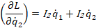

The dynamic equations of the system are finally given by
 (1.4)
(1.4)
 (1.5)
(1.5)
In compact form, the system can be rewritten as follows

(1.6)
where  is the vector of generalized coordinates,
  is the vector of joint torques,
  is the inertia matrix and is given by

(1.7)
and

(1.8)
Note that the matrix is constant and positive definite. The equations of motion are also given by
 (1.9)
(1.9)
 (1.10)
Simulink model

Figure 3.2. Simulation model
5.1. Simulation results
In this section, we present the simulation results using MATLAB and SIMULINK (Figure 3.2).
 and
and  .
.
The initial conditions are


We chose the gains  and
and  and the results are shown in Figure 3.3. The Lyapunov function decreases as expected. The energy converges monotonically to zero. The control input T converges to zero for the first controller (see Figure 3.3). The control input magnitude is acceptable. The phase plots show convergence to the homoc1inic orbit. The closed-loop behavior strongly depends on the controller parameters
  ,
,  and
and  . The parameters used in the simulations have been selected by trying different values.
Figure 3.3: Simulation results
How we did it
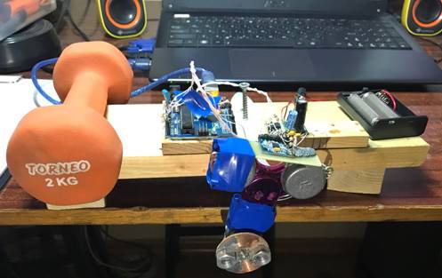
The spinner was attached to a stick (kitchen brush for baking).
On the shaft of the motor soldered a disk cut from the foil of fiberglass (this material is made of boards) to it, in fact, the epoxy glue is glued bolts to increase the mass, and the counterweights to the spinner are glued from the lead fishing cargo.
The accelerometer is positioned so that its X-axis is parallel to the axis on which the pendulum (spinner) is fixed, then the program calculates the rotation and angular velocity with respect to this axis X.
Connect wires from SCL and SDA from the accelerometer, which are each twisted separately with a GND (ground) wire to reduce the effect of interference from the motor.
Accelerometer module - GY-521.
To control the motor, the two-channel driver of the HG7881 engine is used, which is located directly beside the engine on the spinner, and so not separately from outside, because with the driver from outside the current pulses coming from the driver to the motor would flow along long wires and create too much interference interfering the I2C interface, which communicates with the arduin and the accelerometer module.
The driver is powered by a separate source: two Li-ion batteries connected in series, which gives + -8V, which are stabilized to a 5V DC DC / DC voltage step-down converter based on MP1584EN.
The driver is controlled by Arduin with the decoupling of two optocouplers PC817, in order to avoid unnecessary interference from the motor in the power circuit (this disabling the arduinu..).
To start all this, you need to receive data from the accelerometer.
The best option is to use DMP to get accurate data with a high frequency of ~ 200Hz.
The only adequate code that allows to work properly with this accelerometer and using this same DMP is indicated in the next paragraph.
The MPU6050_6Axis_MotionApps20.h library allows you to get a lot of data already processed, but we are particularly interested in: the orientation of the gravity vector relative to the accelerometer, as well as the angular velocity around the X axis.
Project the gravity vector on the XY plane of the accelerometer and obtain the angle of inclination of the pendulum (spinner) relative to the center of the earth.
Using this data further in the program the decision is made that to do the motor.
There were added pull-up resistors on the I2C bus, filter capacitors for power, as well as a pair of capacitors from ground to the motor terminals and grounded its housing. Sam Arduin is powered by the usb port of the computer. the pendulum is started through the terminal on the computer, just to see if the connection with the accelerometer was established, and other real-time data can be monitored during debugging.
Programming code for Arduino
import processing.serial.*;
import processing.opengl.*;
import toxi.geom.*;
import toxi.processing.*;
ToxiclibsSupport gfx;
Serial port;
char[] teapotPacket = new char[14];
int serialCount = 0;
int synced = 0;
int interval = 0;
float[] q = new float[4];
Quaternion quat = new Quaternion(1, 0, 0, 0);
float[] gravity = new float[3];
float[] euler = new float[3];
float[] ypr = new float[3];
void setup() {
size(300, 300, OPENGL);
gfx = new ToxiclibsSupport(this);
lights();
smooth();
println(Serial.list());
String portName = Serial.list()[0];
port = new Serial(this, portName, 115200);
port.write('r');
}
void draw() {
if (millis() - interval > 1000) {
port.write('r');
interval = millis();
}
background(0);
pushMatrix();
translate(width / 2, height / 2);
float[] axis = quat.toAxisAngle();
rotate(axis[0], -axis[1], axis[3], axis[2]);
fill(255, 0, 0, 200);
box(10, 10, 200);
fill(0, 0, 255, 200);
pushMatrix();
translate(0, 0, -120);
rotateX(PI/2);
drawCylinder(0, 20, 20, 8);
popMatrix();
fill(0, 255, 0, 200);
beginShape(TRIANGLES);
vertex(-100, 2, 30); vertex(0, 2, -80); vertex(100, 2, 30);
vertex(-100, -2, 30); vertex(0, -2, -80); vertex(100, -2, 30);
vertex(-2, 0, 98); vertex(-2, -30, 98); vertex(-2, 0, 70);
vertex(2, 0, 98); vertex(2, -30, 98); vertex(2, 0, 70);
endShape();
beginShape(QUADS);
vertex(-100, 2, 30); vertex(-100, -2, 30); vertex(0, -2, -80); vertex(0, 2, -80);
vertex(100, 2, 30); vertex(100, -2, 30); vertex(0, -2, -80); vertex(0, 2, -80);
vertex(-100, 2, 30); vertex(-100, -2, 30); vertex(100, -2, 30); vertex(100, 2, 30);
vertex(-2, 0, 98); vertex(2, 0, 98); vertex(2, -30, 98); vertex(-2, -30, 98);
vertex(-2, 0, 98); vertex(2, 0, 98); vertex(2, 0, 70); vertex(-2, 0, 70);
vertex(-2, -30, 98); vertex(2, -30, 98); vertex(2, 0, 70); vertex(-2, 0, 70);
endShape();
popMatrix();
}
void serialEvent(Serial port) {
interval = millis();
while (port.available() > 0) {
int ch = port.read();
if (synced == 0 && ch!= '$') return; // initial synchronization - also used to resync/realign if needed
synced = 1;
print ((char)ch);
if ((serialCount == 1 && ch!= 2)
|| (serialCount == 12 && ch!= '\r')
|| (serialCount == 13 && ch!= '\n')) {
serialCount = 0;
synced = 0;
return;
}
if (serialCount > 0 || ch == '$') {
teapotPacket[serialCount++] = (char)ch;
if (serialCount == 14) {
serialCount = 0;
q[0] = ((teapotPacket[2] << 8) | teapotPacket[3]) / 16384.0f;
q[1] = ((teapotPacket[4] << 8) | teapotPacket[5]) / 16384.0f;
q[2] = ((teapotPacket[6] << 8) | teapotPacket[7]) / 16384.0f;
q[3] = ((teapotPacket[8] << 8) | teapotPacket[9]) / 16384.0f;
for (int i = 0; i < 4; i++) if (q[i] >= 2) q[i] = -4 + q[i];
quat.set(q[0], q[1], q[2], q[3]);
gravity[0] = 2 * (q[1]*q[3] - q[0]*q[2]);
gravity[1] = 2 * (q[0]*q[1] + q[2]*q[3]);
gravity[2] = q[0]*q[0] - q[1]*q[1] - q[2]*q[2] + q[3]*q[3];
euler[0] = atan2(2*q[1]*q[2] - 2*q[0]*q[3], 2*q[0]*q[0] + 2*q[1]*q[1] - 1);
euler[1] = -asin(2*q[1]*q[3] + 2*q[0]*q[2]);
euler[2] = atan2(2*q[2]*q[3] - 2*q[0]*q[1], 2*q[0]*q[0] + 2*q[3]*q[3] - 1);
ypr[0] = atan2(2*q[1]*q[2] - 2*q[0]*q[3], 2*q[0]*q[0] + 2*q[1]*q[1] - 1);
ypr[1] = atan(gravity[0] / sqrt(gravity[1]*gravity[1] + gravity[2]*gravity[2]));
ypr[2] = atan(gravity[1] / sqrt(gravity[0]*gravity[0] + gravity[2]*gravity[2]));
}
}
}
}
void drawCylinder(float topRadius, float bottomRadius, float tall, int sides) {
float angle = 0;
float angleIncrement = TWO_PI / sides;
beginShape(QUAD_STRIP);
for (int i = 0; i < sides + 1; ++i) {
vertex(topRadius*cos(angle), 0, topRadius*sin(angle));
vertex(bottomRadius*cos(angle), tall, bottomRadius*sin(angle));
angle += angleIncrement;
}
endShape();
if (topRadius!= 0) {
angle = 0;
beginShape(TRIANGLE_FAN);
vertex(0, 0, 0);
for (int i = 0; i < sides + 1; i++) {
vertex(topRadius * cos(angle), 0, topRadius * sin(angle));
angle += angleIncrement;
}
endShape();
}
if (bottomRadius!= 0) {
angle = 0;
beginShape(TRIANGLE_FAN);
vertex(0, tall, 0);
for (int i = 0; i < sides + 1; i++) {
vertex(bottomRadius * cos(angle), tall, bottomRadius * sin(angle));
angle += angleIncrement;
}
endShape();
}
}
Project plan
The baseline project plan and Gant’s diagram are represented at the Figures 5.1 - 5.2.

Figure 5.1. Project plan (1)

Figure 5.2. Project plan (2)
Business plan
Budget and component
| № | Name | Price per one (RUB) |
| Эпоксилный клей Epoxy Metal | ||
| Свинцовые грузы | ||
| Провод Мгтф 2м 0.03мм^2 | ||
| Паяльную кислоту 30ml | ||
| Резисторы 10кОм 10 шт | ||
| Оптопары pc817 4шт. | ||
| Электромотор |
Applicability
At the same time, the Reaction Wheel Pendulum exhibits several properties, such as underactuation and nonlinearity,1 that make it an attractive and useful system for research and advanced education. As such, the Reaction Wheel Pendulum is ideally suited for educating university students at virtually every level, from entering freshman to advanced graduate students.
There are many other examples of control problems in engineering systems where pendulum dynamics provides useful insight, including stabilization of overhead (gantry) cranes, roll stabilization of ships and trucks, and slosh control of liquids. Thus, a study of the pendulum and pendulum-like systems is an excellent starting point to understand issues in nonlinear dynamics and control.
References
1. https://www.youtube.com/watch?v=rPf_6y0g1xk
2. https://www.youtube.com/watch?v=6J7Xby1ChOM
3. https://thl.okstate.edu/
4. Fantoni, I., Lozano, R., «Non-linear Control for Underactuated Mechanical Systems» 295 стр., 2002г.