Квадратичный конгруэнтный метод
zt+1 = (dx2t + axt + c) mod N, t = 0,1,2…
Характеристики (x0, a, c, d, N) Є V4N × N квадратичной конгруэнтной последовательности
Кубический конгруэнтный метод. Последовательность случайных чисел вычисляется с помощью следующего рекуррентного соотношения
Xi+1=(ax3+ax2+ax+d)mod m
Для практических расчетов принимают m=2k, k=14,15,31
1. #include <iostream>
2. using namespace std;
3. double congruential(int &); // прототип функции генерации псевдослучайных чисел
4. int main(int argc, char* argv[])
5. {
6. const int number_numbers = 25; // количество псевдослучайных чисел
7. int x0 = 2; // начальное значение (выбирается случайно 0 <= x0 < m)
8. cout << "\npseudo-random numbers: ";
9. for (int i = 0; i <= number_numbers; i++)
10. cout << congruential(x0) << " "; // генерация i-го числа
11. cout << "\n";
12. system("pause");
13. return 0;
14. }
15. double congruential(int &x) // функция генерации псевдослучайных чисел
16. {
17. const int m = 100, // генерация псевдослучайных чисел в диапазоне значений от 0 до 100 выбирается случайно m > 0)
18. a = 8, // множитель (выбирается случайно 0 <= a <= m)
19. inc = 65; // инкрементирующее значение (выбирается случайно 0 <= inc <= m)
20. x = ((a * x) + inc) % m; // формула линейного конгруэнтного метода генерации псевдослучайных чисел
21. return (x / double(m));
22. }
|
| 8 Random numbers in C++. John von Neumann's pseudorandom number generator. C++ implementation. 1
The procedure, received the name of the middle squares (was proposed by von Neumann and Metropolis in the 1940s).
The algorithm for obtaining a sequence of random numbers by the middle squares method is as follows:
Let there be a 2n-bit number less than Xi+1=0,а1,а2,…а2n
Erect it in a square:
X2i=0,b1,b2,…b4n
and then take the average of 2n digits:
Xi+1=0, bn+1,bn+2,…b3n
which will be the next number.
For example: X0=0,2152, X20=0,04631104, hence X1=0,6311;
X21=0,39828721 hence X1=0,8287 etc.
The disadvantage of this method is that there is a correlation between the sequence numbers, and in some cases there may be no accident at all.
The method of median squares is not accidental, that is, unpredictable (this is the most significant drawback). In fact, if we know one number, the next number is completely predefined, because the rules for getting it invariably. In fact, when x 0 is specified, the entire sequence of numbers xi is predetermined. This remark applies to all arithmetic generators.
| 8 случайных чисел в C++. Генератор псевдослучайных чисел Джона фон Неймана. Реализации C++. 1
Процедура, получившая, название серединных квадратов (была предложена фон Нейманом и Метрополисом в 1940-х годах).
Алгоритм получения последовательности случайных чисел методом серединных квадратов сводится к следующему:
Пусть имеется 2 n -разрядное число, меньше 1: Xi+1=0,а1,а2,…а2n
Возведем его в квадрат:
X2i=0,b1,b2,…b4n
а затем возьмем средние 2 n разрядов:
Xi+1=0, bn+1,bn+2,…b3n
которые и будут очередным числом. Например: X0=0,2152, X20=0,04631104, отсюда X1=0,6311;
X21=0,39828721 отсюда X1=0,8287 и т.д.
Недостатком этого метода является наличие корреляции между числами последовательности, а в ряде случаев случайность вообще может отсутствовать.
Метод срединных квадратов вовсе не является случайным, то есть непредсказуемым (это наиболее существенный его недостаток). На самом деле, если мы знаем одно число, следующее число является полностью предопределенным, поскольку правило его получения неизменно. Фактически, когда задается х 0, предопределяется вся последовательность чисел xi. Это замечание касается всех арифметических генераторов.
|
| 9 Write the code for prime factorization using the simple trial division method. 1
9 Напишите код для простой факторизации, используя простой метод пробного деления. 1
Enumeration of divisor (trial division) — the algorithm of factorization or testing Prime numbers by exhaustive search of all potential divisors. Too much of the factors is the algorithm used to determine what number is in front of us: simple or compound.
The algorithm consists in the sequential division of a given positive integer number into all integers, starting with two and ending with a value less than or equal to the square root of the tested number. If at least one divisor divides the tested number without remainder, it is a composite number. If you have tested the number there is no divider that divides it without a remainder, then that number is Prime.
| 9 Напишите код для простой факторизации, используя простой метод пробного деления. 1
Не работает
9 Write the code for prime factorization using the simple trial division method.
Перебор делителей (пробное деление) — алгоритм факторизации или тестирования простоты числа путём полного перебора всех возможных потенциальных делителей. Перебор делителей – это алгоритм, применяемый для определения, какое число перед нами: простое или составное.
Алгоритм заключается в последовательном делении заданного натурального числа на все целые числа, начиная с двойки и заканчивая значением меньшим или равным квадратному корню тестируемого числа. Если хотя бы один делитель делит тестируемое число без остатка, то оно является составным. Если у тестируемого числа нет ни одного делителя, делящего его без остатка, то такое число является простым.
|
| 10 Fibonacci generator (LFG or sometimes LFib) pseudorandom number generator. C++ implementation. 1
Fibonacci numbers - elements of a numerical sequence in which each subsequent number is equal to the sum of two previous numbers
Пример: 0, 1, 1, 2, 3, 5, 8, 13, 21, 34, 55, 89, 144, 233, 377, 610, 987, 1597, 2584, 4181, 6765, 10946... Formula: F(n+2)=Fn+F(n+1)
Fibonacci Generator. The sequence of random numbers is calculated using the following recurrent relation Xi+1=(xi+xi-1)mod m
where xi and xi-1 are integers lying between zero and m. For practical calculations take m=2K, k=14,15,31
1. #include <iostream>
2. using namespace std;
3. int Fib(int i)
4. {
5. int value = 0;
6. if(i < 1) return 0;
7. if(i == 1) return 1;
8. return Fib(i-1) + Fib(i - 2);
9. }
10. int main()
11. {
12. int i = 0;
13. while(i < 47)
14. {
15. cout << Fib(i) << endl;
16. i++;
17. }
18. return 0;
19. }
| 10.Чи́сла Фибона́ччи — элементы числовой последовательности в которой каждое последующее число равно сумме двух предыдущих чисел. Пример: 0, 1, 1, 2, 3, 5, 8, 13, 21, 34, 55, 89, 144, 233, 377, 610, 987, 1597, 2584, 4181, 6765, 10946... Формула: F(n+2)=Fn+F(n+1)
Генератор Фибоначчи.Последовательность случайных чисел вычисляется с помощью следующего рекуррентного соотношения Xi+1=(xi+xi-1)mod m
где xi и xi-1 - целые числа, лежащие между нулем и m. Для практических расчетов принимают m=2k, k=14,15,31
https://function-x.ru/cpp_ryad_chisel_fibonacci.html
Наиболее простая реализация для рядов чисел Фибоначчи с целочисленным типом данных выглядит так:
Код C++
20. #include <iostream>
21. using namespace std;
22. int Fib(int i)
23. {
24. int value = 0;
25. if(i < 1) return 0;
26. if(i == 1) return 1;
27. return Fib(i-1) + Fib(i - 2);
28. }
29. int main()
30. {
31. int i = 0;
32. while(i < 47)
33. {
34. cout << Fib(i) << endl;
35. i++;
36. }
37. return 0;
38. }
Как уже отмечалось, есть разница, используется ли тип данных int или long int: в первом случае для того, чтобы вычислить и вывести на экран весь ряд чисел Фибоначчи до 46-го включительно, требуется около 40 минут, а во втором - примерно на треть меньше.
Код C++
1. #include <iostream>
2. using namespace std;
3. long int Fib(int i)
4. {
5. int value = 0;
6. if(i < 1) return 0;
7. if(i == 1) return 1;
8. return Fib(i-1) + Fib(i - 2);
9. }
10. long int main()
11. {
12. int i = 0;
13. while(i < 47)
14. {
15. cout << Fib(i) << endl;
16. i++;
17. }
18. return 0;
19. }
Можно добиться и большего максимального значения, если определить тип данных как unsigned (без знака). Если максимальное значение для signed long int (то есть со знаком, используется по умолчанию) составляет 2 147 483 647, то для unsigned long int оно составляет 4 294 967 295. Ниже приведён код такой реализации для ряда чисел Фибоначчи.
Код C++
1. #include <iostream>
2. using namespace std;
3. int Fib(int Place)
4. {
5. unsigned long OldValue = 0;
6. unsigned long Value = 1;
7. unsigned long Hold;
8. if(i < 1){return(0);}
9. for(int n = 1; n < Place;n++)
10. {
11. Hold = Value;
12. Value+=OldValue;
13. OldValue = Hold;
14. }
15. return(Value);
16. }
Функция для рядов чисел Фибоначчи с условием значения double для членов последовательности выглядит так:
Код C++
1. #include <iostream>
2. using namespace std;
3. double fib(int place)
4. {
5. static double* lookup = NULL;
6. if(lookup == NULL)
7. {
8. lookup = new double[300];
9. lookup[0] = 0;
10. lookup[1] = 1;
11. for(int i = 2; i < 300; ++i)
12. {
13. lookup[i] = lookup[i - 1] + lookup[i - 2];
14. }
15. }
16. if(place < 300)
17. {
18. return lookup[place];
19. }
20. return fib(place - 1) + fib(place - 2);
21. }
Далее - способ отойти от компактности программы в пользу функциональности (пользователь имеет возможность определять, сколько членов последовательности Фибоначчи нужно вычислить и вывести, но максимальное значение определено типом int, так что возможны модификации с другими типами данных):
Код C++
#include <iostream>
using namespace std;
int Fib(int i)
{
int f1 = 0;
int f2 = 1;
int fn;
if (i < 1) { return 0; }
if (i == 1){ cout << "0 1\n"; }
if (i > 1)
{
cout << "0 1 ";
for (int j = 1; j < i;j++)
{
fn = f1 + f2;
cout << fn << " ";
f1 = f2;
f2 = fn;
}
}
cout << "\n\n";
return 0;
};
int main()
{
char choice;
int input;
cout << "Enter how long you wish the Fibanacci series to display: ";
cin >> input;
Fib(input);
cout << "Again? Y/N: ";
cin >> choice;
while (choice == 'y' || choice == 'Y')
|
11 Implement the Box–Muller transform which is a pseudo-random number sampling method for generating pairs of independent, standard, normally distributed (zero expectation, unit variance) random numbers, given a source of uniformly distributed random numbers. 1
Box-Mueller transformation is a method of modeling standard normally distributed random variables. Has two options. The method is accurate, unlike, for example, methods based on the Central limit theorem.
Let r and  be independent random variables uniformly distributed over the interval (0,1]. We compute z0 and z1 by formulas be independent random variables uniformly distributed over the interval (0,1]. We compute z0 and z1 by formulas 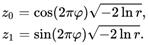 Then z0 and z1 will be independent and normally distributed with expectation 0 and variance 1. When implemented on a computer it is usually faster not to calculate both trigonometric functions — cos and sin — but to calculate one of them through another. It is even better to use the second variant of the Mueller — Box transformation instead.
Second option
Let x and y be independent random variables uniformly distributed on the interval [-1,1]. We compute s=x2 + y2. If it turns out that s>1 or s=0, the x and y values should be "discarded" and regenerated. Once condition 0<s<1 is satisfied, by formulas
Then z0 and z1 will be independent and normally distributed with expectation 0 and variance 1. When implemented on a computer it is usually faster not to calculate both trigonometric functions — cos and sin — but to calculate one of them through another. It is even better to use the second variant of the Mueller — Box transformation instead.
Second option
Let x and y be independent random variables uniformly distributed on the interval [-1,1]. We compute s=x2 + y2. If it turns out that s>1 or s=0, the x and y values should be "discarded" and regenerated. Once condition 0<s<1 is satisfied, by formulas   we should calculate z0 and z1 which, as in the first case, will be independent quantities satisfying the standard normal distribution.
The coefficient of use of basic random variables for the first variant is obviously equal to one. For the second variant, it is the ratio of the circumference of a unit radius to the square with side two, that is
we should calculate z0 and z1 which, as in the first case, will be independent quantities satisfying the standard normal distribution.
The coefficient of use of basic random variables for the first variant is obviously equal to one. For the second variant, it is the ratio of the circumference of a unit radius to the square with side two, that is  however, in practice the second variant is usually faster, due to the fact that it uses only one transcendental function, ln(.) Is an advantage for most implementations outweigh the need of generating a larger number of uniformly distributed random variables. however, in practice the second variant is usually faster, due to the fact that it uses only one transcendental function, ln(.) Is an advantage for most implementations outweigh the need of generating a larger number of uniformly distributed random variables.
| Реализуйте преобразование Box-Muller, которое является методом выборок псевдослучайных чисел для генерации пар независимых, стандартных, нормально распределенных (нулевое ожидание, единичная дисперсия) случайных чисел, с учетом источника равномерно распределенных случайных чисел. 1  Преобразование Бокса — Мюллера — метод моделирования стандартных нормально распределённых случайных величин. Имеет два варианта. Метод является точным, в отличие, например, от методов, основывающихся на центральной предельной теореме.
Пусть r{\displaystyle r} и {\displaystyle \varphi \ } — независимые случайные величины, равномерно распределённые на интервале {\displaystyle (0,\;1]}(0,1]. Вычислим {\displaystyle z_{0}}z0 и {\displaystyle z_{1}}z1 по формулам
Преобразование Бокса — Мюллера — метод моделирования стандартных нормально распределённых случайных величин. Имеет два варианта. Метод является точным, в отличие, например, от методов, основывающихся на центральной предельной теореме.
Пусть r{\displaystyle r} и {\displaystyle \varphi \ } — независимые случайные величины, равномерно распределённые на интервале {\displaystyle (0,\;1]}(0,1]. Вычислим {\displaystyle z_{0}}z0 и {\displaystyle z_{1}}z1 по формулам
 {\displaystyle z_{0}=\cos(2\pi \varphi){\sqrt {-2\ln r}},}
{\displaystyle z_{1}=\sin(2\pi \varphi){\sqrt {-2\ln r}}.}
Тогда {\displaystyle z_{0}}z0 и {\displaystyle z_{1}}z1 будут независимы и распределены нормально с математическим ожиданием 0 и дисперсией 1. При реализации на компьютере обычно быстрее не вычислять обе тригонометрические функции — {\displaystyle \cos(\cdot)}cos и {\displaystyle \sin(\cdot)}sin — а рассчитать одну из них через другую. Ещё лучше воспользоваться вместо этого вторым вариантом преобразования Бокса — Мюллера.
Второй вариант
Пусть x{\displaystyle x} и y{\displaystyle y} — независимые случайные величины, равномерно распределённые на отрезке {\displaystyle [-1,\;1]}[-1,1]. Вычислим {\displaystyle {s=x^{2}+y^{2}}}s=x2+y2. Если окажется, что {\displaystyle {s>1}}s>1 или {\displaystyle {s=0}}s=0, то значения {\displaystyle x}x и {\displaystyle y}y следует «выбросить» и сгенерировать заново. Как только выполнится условие {\displaystyle {0<s\leqslant 1}}0<s<1, по формулам {\displaystyle z_{0}=\cos(2\pi \varphi){\sqrt {-2\ln r}},}
{\displaystyle z_{1}=\sin(2\pi \varphi){\sqrt {-2\ln r}}.}
Тогда {\displaystyle z_{0}}z0 и {\displaystyle z_{1}}z1 будут независимы и распределены нормально с математическим ожиданием 0 и дисперсией 1. При реализации на компьютере обычно быстрее не вычислять обе тригонометрические функции — {\displaystyle \cos(\cdot)}cos и {\displaystyle \sin(\cdot)}sin — а рассчитать одну из них через другую. Ещё лучше воспользоваться вместо этого вторым вариантом преобразования Бокса — Мюллера.
Второй вариант
Пусть x{\displaystyle x} и y{\displaystyle y} — независимые случайные величины, равномерно распределённые на отрезке {\displaystyle [-1,\;1]}[-1,1]. Вычислим {\displaystyle {s=x^{2}+y^{2}}}s=x2+y2. Если окажется, что {\displaystyle {s>1}}s>1 или {\displaystyle {s=0}}s=0, то значения {\displaystyle x}x и {\displaystyle y}y следует «выбросить» и сгенерировать заново. Как только выполнится условие {\displaystyle {0<s\leqslant 1}}0<s<1, по формулам  и и 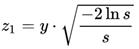 следует рассчитать z0 и z1 которые, как и в первом случае, будут независимыми величинами, удовлетворяющими стандартному нормальному распределению.
Коэффициент использования базовых случайных величин для первого варианта, очевидно, равен единице. Для второго варианта это отношение площади окружности единичного радиуса к площади квадрата со стороной два, то есть следует рассчитать z0 и z1 которые, как и в первом случае, будут независимыми величинами, удовлетворяющими стандартному нормальному распределению.
Коэффициент использования базовых случайных величин для первого варианта, очевидно, равен единице. Для второго варианта это отношение площади окружности единичного радиуса к площади квадрата со стороной два, то есть  Тем не менее, на практике второй вариант обычно оказывается быстрее, за счёт того, что в нём используется только одна трансцендентная функция, ln(.) Это преимущество для большинства реализаций перевешивает необходимость генерации большего числа равномерно распределённых случайных величин.{\displaystyle \pi /4\approx 0{,}785} Тем не менее, на практике второй вариант обычно оказывается быстрее, за счёт того, что в нём используется только одна трансцендентная функция, ln(.) Это преимущество для большинства реализаций перевешивает необходимость генерации большего числа равномерно распределённых случайных величин.{\displaystyle \pi /4\approx 0{,}785}
|
| 12 Implement the Euler-Cromer's algorithm of solving the time-independent Schrodinger equation. 1
| 12. Реализовать алгоритм Эйлера-Кромера решения не зависящего от времени уравнения Шредингера. 1 (y! в правых точках)

 1. #include <iostream>
2. #include <cmath>
3. #include <fstream>
4. #include <iomanip>
5. using namespace std;
6. float V (float x){ float a=3.0, V0=5.0, D=0.001;
7. float f; if(abs(x)<a){f=0;}
8. else {f=V0;} return f;}
9. int main(){
10. ofstream myfile;
11. myfile.open("Shredinger.dat");
12. float x_target=2;
13. float e_psilon=0.001;
14. float En_target=0;
15. for(float En=0.806601; En<=0.806701; En+=.0001){
16. float phi=1.0, phi_p=0.0, dx=0.01, a=3.0, En=0.137;
17. for(float x=0.0; x<=a*1.1; x+=dx){
18. //if(x>=abs(a)){phi=0;}//(x<xn+dx)&&(abs(psi)<=e_psilon)){
19. cout<<"*"<<En<<"*"; En_target+dx)&&"\n"<<En<<"\n";
20. for (float x=0.0; x<=2.2; x+=dx){
21. float phi2p=-2*(En-V(x))*phi;
22. phi_p=phi_p+phi2p*dx;
23. phi=phi+phi_p*dx;
24. cout << x << "\t" << phi << "\n";
25. cout << -x << "\t" << phi << "\n";
26. myfile << x << "\t" << phi << "\n";
27. myfile << -x << "\t" << phi << "\n";
28. }
29. return 0; }
1. #include <iostream>
2. #include <cmath>
3. #include <fstream>
4. #include <iomanip>
5. using namespace std;
6. float V (float x){ float a=3.0, V0=5.0, D=0.001;
7. float f; if(abs(x)<a){f=0;}
8. else {f=V0;} return f;}
9. int main(){
10. ofstream myfile;
11. myfile.open("Shredinger.dat");
12. float x_target=2;
13. float e_psilon=0.001;
14. float En_target=0;
15. for(float En=0.806601; En<=0.806701; En+=.0001){
16. float phi=1.0, phi_p=0.0, dx=0.01, a=3.0, En=0.137;
17. for(float x=0.0; x<=a*1.1; x+=dx){
18. //if(x>=abs(a)){phi=0;}//(x<xn+dx)&&(abs(psi)<=e_psilon)){
19. cout<<"*"<<En<<"*"; En_target+dx)&&"\n"<<En<<"\n";
20. for (float x=0.0; x<=2.2; x+=dx){
21. float phi2p=-2*(En-V(x))*phi;
22. phi_p=phi_p+phi2p*dx;
23. phi=phi+phi_p*dx;
24. cout << x << "\t" << phi << "\n";
25. cout << -x << "\t" << phi << "\n";
26. myfile << x << "\t" << phi << "\n";
27. myfile << -x << "\t" << phi << "\n";
28. }
29. return 0; }
|
| 13 Implement the Euler-Cromer's algorithm of solving the time-independent Schrodinger equation. Calculate an energy spectrum for the particle in the square potential box. 1
|
|
| 14 Implement the Euler-Cromer's algorithm of solving the time-independent Schrodinger equation. Calculate a set of eigenfunctions for the particle in the square potential box. 1
| Шредингера. Вычислить набор собственных функций для частицы в квадрате потенциала потенциала.
|
15 Implement the Picard iterative process to solve differential equations. 1
The Picard method or the Picard method of successive approximations is known from the course of ordinary differential equations. Using this method, the approximate solution of the Cauchy problem is obtained analytically as a sequence of approximations  to the solution y(x) as follows: to the solution y(x) as follows:  y0 (x) – given.
We show the application of the Picard method in the following example.
Example 3. Find three consecutive approximations of the solution of the equation y0 (x) – given.
We show the application of the Picard method in the following example.
Example 3. Find three consecutive approximations of the solution of the equation
 with the initial condition y(0)=0 Solution. Taking into account the initial condition, we replace the food with an integral ordinary differential equation: with the initial condition y(0)=0 Solution. Taking into account the initial condition, we replace the food with an integral ordinary differential equation:  as the initial approximation we choose y 0=x(0). We construct the first approximation: as the initial approximation we choose y 0=x(0). We construct the first approximation:   then we construct the second and third approximations: then we construct the second and third approximations: 

 Due to the fact that f(x,y)=x+y is defined and continuous in the whole plane, any numbers can be taken as Փ and Փ, for example, a=1, b=0.5 Then the following estimates are valid:

 from Here we find from Here we find  As a result, the gap [0;0,33] have the estimate:
  and therefore, and therefore,


| 15 реализовать итерационный процесс Пикара для решения дифференциальных уравнений. 1
https://www.math.tsu.ru/EEResources/pdf_common/difference_schemes_theory_2014.pdf
Метод Пикара или метод последовательных приближений Пикара известен из курса обыкновенных дифференциальных уравнений. С помощью этого метода приближённое решение задачи Коши получается в аналитическом виде как последовательность приближений к решению y(x) следующим образом:  y0 (x) – задано.
Покажем применение метода Пикара на следующем примере. Пример 3. Найти три последовательных приближения решения уравнения
с начальным условием y(0)=0 Решение. С учётом начального условия заменим ОДУ интегральным: y0 (x) – задано.
Покажем применение метода Пикара на следующем примере. Пример 3. Найти три последовательных приближения решения уравнения
с начальным условием y(0)=0 Решение. С учётом начального условия заменим ОДУ интегральным:  В качестве начального приближения выберем y0=x(0). Построим первое приближение: В качестве начального приближения выберем y0=x(0). Построим первое приближение:   Далее построим второе и третье приближения: Далее построим второе и третье приближения:  
 В силу того что f(x,y)=x+y определена и непрерывна во всей плоскости, в качестве a и b можно брать любые числа, например, a=1, b=0.5. Тогда справедливы следующие оценки: В силу того что f(x,y)=x+y определена и непрерывна во всей плоскости, в качестве a и b можно брать любые числа, например, a=1, b=0.5. Тогда справедливы следующие оценки:    Отсюда находим Отсюда находим  В результате на промежутке [0;0,33] имеет место оценка:
 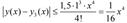 и, следовательно, и, следовательно,  Рабочая программа с уроков
1. #include <iostream>
2. #include <cmath>
3. #include <fstream>
4. #include <iomanip>
5. using namespace std;
6. float f(float x, float y) {
7. return(x*x-y*y);}
8. float sq1(float a, float b, float dx, float y) {
9. float S=0; float x = a;
10. while(x<=b){S+= (f(x,y)+f(x+dx,y))*dx/2.0; x+=dx;}
11. return S;}
12. float e_xact(float x){
13. // return (pow(x,3.0)/3.0+pow(x,7.0)/63.0+2.0*pow(x,11.0)/2079.0+pow(x,15.0)/59525.0);
14. return (1-x+pow(x, 2.0)-pow(x,3.0)/3.0+pow(x,4.0)/24.0);
15. }
16. int main()
17. {
18. cout<<setprecision(3);
19. float x0=0.0, y0=1.0, y=y0, dx=0.0001;
20. for(float x=0.0;x<=2.0;x+=0.1){
21. for(int i=0; i<=1000; i++){
22. y=y0+sq1(x0, x, dx, y);
23. }
24. cout<<x<<"\t"<<y<< "\t" <<e_xact(x)<< "\n";
25. }
26. }
Рабочая программа с уроков
1. #include <iostream>
2. #include <cmath>
3. #include <fstream>
4. #include <iomanip>
5. using namespace std;
6. float f(float x, float y) {
7. return(x*x-y*y);}
8. float sq1(float a, float b, float dx, float y) {
9. float S=0; float x = a;
10. while(x<=b){S+= (f(x,y)+f(x+dx,y))*dx/2.0; x+=dx;}
11. return S;}
12. float e_xact(float x){
13. // return (pow(x,3.0)/3.0+pow(x,7.0)/63.0+2.0*pow(x,11.0)/2079.0+pow(x,15.0)/59525.0);
14. return (1-x+pow(x, 2.0)-pow(x,3.0)/3.0+pow(x,4.0)/24.0);
15. }
16. int main()
17. {
18. cout<<setprecision(3);
19. float x0=0.0, y0=1.0, y=y0, dx=0.0001;
20. for(float x=0.0;x<=2.0;x+=0.1){
21. for(int i=0; i<=1000; i++){
22. y=y0+sq1(x0, x, dx, y);
23. }
24. cout<<x<<"\t"<<y<< "\t" <<e_xact(x)<< "\n";
25. }
26. }
|
| 16 Partial differential equations. Canonical form reduction. Boundary problems. 1
| 29. Дифференциальное уравнение. Каноническая редукция формы. Краевая задача. 1
|
| 17 Laplace PDE. Finite differences scheme and numerical solution. 1
|
|
| 18 Laplace PDE. Finite differences scheme and numerical solution. Relaxation method. 1
|
|
19 Lagrange interpolating polynomial C++ implementation. 1
The sample of experimental data is an array of data that characterizes the process of changing the measured signal for a given time (or relative to another variable). To perform a theoretical analysis of the measured signal, it is necessary to find an approximating function that will link a discrete set of experimental data with a continuous function - an n-degree interpolation polynomial. One of the ways of representing the interpolation polynomial of n-degree can be used the polynomial in the Lagrange form.
An interpolation polynomial in the form of a Lagrangian is a mathematical function that allows you to write an n-degree polynomial that will connect all the given points from a set of values obtained experimentally or by random sampling at different times with a non-constant time step of measurements.
1. The interpolation formula of Lagrange
In General, the interpolation polynomial in the Lagrange form is written as follows:  where n is the degree of polynomial L(x);
f (xi) value of the interpolating function f(xi) at point xi;
li (x) basis polynomials (Lagrange multiplier), which are defined by
where n is the degree of polynomial L(x);
f (xi) value of the interpolating function f(xi) at point xi;
li (x) basis polynomials (Lagrange multiplier), which are defined by 
 For example, an interpolation polynomial in the Lagrange form, passing through three given points, will be written as follows:


 1. #include <iostream>
2. #include <cmath>
3. #include <fstream>
4. #include <iomanip>
5. using namespace std;
6. int main()
7. { ofstream myfile;
8. for(float xp=0.9; xp<=5.1; xp+=0.1){
9. float x [4] = {1.0,2.0,3.0,5.0};
10. float y [4] = {1.0,5.0,14.0,81.0};
11. float L=0.0;
12. for(int i=0; i<=3; i++){
13. float P=1.0;
14. for(int j=0; j<=3; j++){
15. if(i!=j){
16. P=P*(xp-x[j])/(x[i]-x[j]);
17. }
18. }
19. L=L+P*y[i];
20. }
21. cout«xp «"\t"«L«"\n";
22. }
23. myfile.open("Lagrange1.txt");
24. return 0;
25. }
1. #include <iostream>
2. #include <cmath>
3. #include <fstream>
4. #include <iomanip>
5. using namespace std;
6. int main()
7. { ofstream myfile;
8. for(float xp=0.9; xp<=5.1; xp+=0.1){
9. float x [4] = {1.0,2.0,3.0,5.0};
10. float y [4] = {1.0,5.0,14.0,81.0};
11. float L=0.0;
12. for(int i=0; i<=3; i++){
13. float P=1.0;
14. for(int j=0; j<=3; j++){
15. if(i!=j){
16. P=P*(xp-x[j])/(x[i]-x[j]);
17. }
18. }
19. L=L+P*y[i];
20. }
21. cout«xp «"\t"«L«"\n";
22. }
23. myfile.open("Lagrange1.txt");
24. return 0;
25. }
| 19 Lagrange interpolating polynomial C++ implementation. 1
19 реализация интерполирующего полинома Лагранжа C++. 1
https://simenergy.ru/math-analysis/digital-processing/76-lagrange-polynomial
Выборка экспериментальных данных представляет собой массив данных, который характеризует процесс изменения измеряемого сигнала в течение заданного времени (либо относительно другой переменной). Для выполнения теоретического анализа измеряемого сигнала необходимо найти аппроксимирующую функцию, которая свяжет дискретный набор экспериментальных данных с непрерывной функцией - интерполяционным полиномом n-степени. Одним из способов представления данного интерполяционного полинома n-степени может быть использован многочлен в форме Лагранжа.
Интерполяционный многочлен в форме Лагранжа– это математическая функция позволяющая записать полином n-степени, который будет соединять все заданные точки из набора значений, полученных опытным путём или методом случайной выборки в различные моменты времени с непостоянным временным шагом измерений.
1. Интерполяционная формула Лагранжа
В общем виде интерполяционный многочленв форме Лагранжа записывается в следующем виде:  где n ˗ степень полинома L(x);
f(xi) ˗ значение значения интерполирующей функции f(xi) в точке xi;
li(x) ˗ базисные полиномы (множитель Лагранжа), которые определяются по формуле:
где n ˗ степень полинома L(x);
f(xi) ˗ значение значения интерполирующей функции f(xi) в точке xi;
li(x) ˗ базисные полиномы (множитель Лагранжа), которые определяются по формуле:  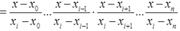 Так, например, интерполяционный многочленв форме Лагранжа, проходящий через три заданных точки, будет записываться в следующем виде: Так, например, интерполяционный многочленв форме Лагранжа, проходящий через три заданных точки, будет записываться в следующем виде: 
  #include <iostream> #include <cmath> #include <fstream> #include <iomanip> using namespace std; int main() { ofstream myfile; for(float xp=0.9; xp<=5.1; xp+=0.1){ float x [4] = {1.0,2.0,3.0,5.0}; float y [4] = {1.0,5.0,14.0,81.0}; float L=0.0; for(int i=0; i<=3; i++){ float P=1.0; for(int j=0; j<=3; j++){ if(i!=j){ P=P*(xp-x[j])/(x[i]-x[j]); } } L=L+P*y[i]; } cout«xp «"\t"«L«"\n"; } myfile.open("Lagrange1.txt"); return 0; }
|
| 20 Newton's "First" Interpolation Formulae (Newton Forward Divided Difference Formula). C++ implementation. 1
| 20" первые " Интерполяционные Формулы Ньютона (Формула разности Ньютона вперед). Реализации C++. 1
Рабочая программа с уроков. Не знаю вперед или назад?
1. #include <iostream>
2. #include <cmath>
3. #include <fstream>
4. #include <iomanip>
5. using namespace std;
6. int main() {
7. ofstream myfile;
8. myfile.open("Nuton formula.dat");
9. for(float xp=1.8; xp<=2.8; xp+=0.01){
10. float x[11]={1.8, 1.9, 2, 2.1, 2.2, 2.3, 2.4, 2.5, 2.6, 2.7, 2.8};
11. float ydy[11][11];
12. float yn;
13. //yn=(1/sqrt(2*3.14))*exp(-(xp*xp/2));
14. ydy[0][0]=0.0794, ydy[1][0]=0.0660, ydy[2][0]=0.0540, ydy[3][0]=0.0440, ydy[4][0]=0.0355, ydy[5][0]=0.0283,
15. ydy[6][0]=0.0224, ydy[7][0]=0.0175, ydy[8][0]=0.0140, ydy[9][0]=0.0105, ydy[10][0]=0.0080;
16. for(int i= 1.0; i<=6.0; i++){
17. for(int j= 0.0; j<=7.0-i; j++){
18. ydy[j][i]=ydy[j+1][i-1]-ydy[j][i-1];}}
19. float Pn=ydy[0][0]; float dx=0.1;
20. for(int i=1.0; i<=6.0; i++){
21. float p = 1.0f;
22. for(int j = 0.0; j<=i-1.0; j++){
23. p=p*(xp-x[j])/((j+1.0)*dx);}
24. Pn=Pn+p*ydy[0][i];
25. yn=(1/sqrt(2*3.14))*exp(-(xp*xp/2));
26. }
27. << xp << " " << Pn << " " << yn << "\n";
28. myfile << xp << " " << Pn << " " << yn << "\n";
29. }
30. return 0; }
|
| 21 Numerical solution of the system of ordinary differential equations. Code examples. 2
|
|
| 22 Numerical solution of the differential equation of the 2-nd order and higher. Code examples. 2
|
|
| 23 C++ user defined functions. Code examples. 2
|
|
| 24 Nonlinear differential equations. Stability of numerical solution. Code examples. 2
|
|
| 25 Partial differential equations. Types of Equations. A simple algorithm for numerical solution. Code examples. 2
| A relation between the dependent variable and independent variable and derivative of the dependent variable is called differential equation. If the derivative present in a differential equation are all ordinary derivatives, then the differential equation is called an ordinary differential equation and if the derivative present in a differential equation are all partial derivatives, then the differential equation is called partial differential equation.
-
 2. If f is a function of two independent variables x and y then,  is a partial differential equation.
Order and Degree of the Differential Equation
The highest order derivative which is presents in the differential equation is called the order of the differential equation and the degree differential equation is the positive integral power to which the highest order derivative present in the equation is raised. In short, the power of the highest order derivative is called the degree of differential equation.
First order differential equations.
- Простейшие дифференциальные уравнения первого порядка вида The simplest first order differential equations of the form y!=f(x) example y!=y+ex , g(x) y!=g(x) example ex y!=sin x
- Differential equations with separable variables of the form Дифференциальные уравнения с разделяющимися переменными вида f1(y) g1(x)dy=f2(y)g2(x)dx or f1(x)g1(x)y!=f2(y)g2(x) example eydy=(x+sin2x)dx
Дифференциальные уравнения с разделенными переменными.
Differential equations with separated variables. f(y)dy=g(x)dx eydy=(x+sin2x)dx
- Линейные неоднородные дифференциальные уравнения первого порядка
- -Linear inhomogeneous first order differential equations y!+P(x)y=Q(x)
y!-xy=-(1+x)e-x
- Дифференциальное уравнение Бернулли
Bernoulli differential equation
y!+P(x)y=Q(x)ya
Модифицированный эйлер
30. #include <iostream>
31. #include <cmath>
32. using namespace std;
33. double F(double x, double y){
34. return x*x-2*y;
35. }
36. int main() {
37. double a=0; double b=10; double h=0.01;
38. double n=(b-a)/h;
39. double x[(int)n];
40. double yp[(int)n];
41. double y[(int)n];
42. //calculate
43. x[0]=a; y[0]=1;
44. cout.width(12);
45. cout << "x[0]="<<a <<" "<< "y[0]="<<b;"\n";
46. for(int i=1; i<=n; i++)
47. {
48. x[i]=a+i*h;
49. yp[i]=y[i-1]+h*F(x[i-1],y[i-1]);
50. y[i]=y[i-1]+h*(F(x[i-1],y[i-1])+F(x[i],yp[i]))/2.0;
51. cout << "x["<<i<<"]="<<x[i] <<" "<< "y["<<i<<"]="<<y[i] << "\n";
52. cout << endl;
53. cout.width(12);
54. }
55. return 0;
56. } is a partial differential equation.
Order and Degree of the Differential Equation
The highest order derivative which is presents in the differential equation is called the order of the differential equation and the degree differential equation is the positive integral power to which the highest order derivative present in the equation is raised. In short, the power of the highest order derivative is called the degree of differential equation.
First order differential equations.
- Простейшие дифференциальные уравнения первого порядка вида The simplest first order differential equations of the form y!=f(x) example y!=y+ex , g(x) y!=g(x) example ex y!=sin x
- Differential equations with separable variables of the form Дифференциальные уравнения с разделяющимися переменными вида f1(y) g1(x)dy=f2(y)g2(x)dx or f1(x)g1(x)y!=f2(y)g2(x) example eydy=(x+sin2x)dx
Дифференциальные уравнения с разделенными переменными.
Differential equations with separated variables. f(y)dy=g(x)dx eydy=(x+sin2x)dx
- Линейные неоднородные дифференциальные уравнения первого порядка
- -Linear inhomogeneous first order differential equations y!+P(x)y=Q(x)
y!-xy=-(1+x)e-x
- Дифференциальное уравнение Бернулли
Bernoulli differential equation
y!+P(x)y=Q(x)ya
Модифицированный эйлер
30. #include <iostream>
31. #include <cmath>
32. using namespace std;
33. double F(double x, double y){
34. return x*x-2*y;
35. }
36. int main() {
37. double a=0; double b=10; double h=0.01;
38. double n=(b-a)/h;
39. double x[(int)n];
40. double yp[(int)n];
41. double y[(int)n];
42. //calculate
43. x[0]=a; y[0]=1;
44. cout.width(12);
45. cout << "x[0]="<<a <<" "<< "y[0]="<<b;"\n";
46. for(int i=1; i<=n; i++)
47. {
48. x[i]=a+i*h;
49. yp[i]=y[i-1]+h*F(x[i-1],y[i-1]);
50. y[i]=y[i-1]+h*(F(x[i-1],y[i-1])+F(x[i],yp[i]))/2.0;
51. cout << "x["<<i<<"]="<<x[i] <<" "<< "y["<<i<<"]="<<y[i] << "\n";
52. cout << endl;
53. cout.width(12);
54. }
55. return 0;
56. }
|
| 26 Boundary conditions and their definition in numerical solution of differential equations. Code examples. 2
Boundary conditions and their definition in the numerical solution of differential equations.
For the numerical solution of ordinary differential equations distinguish problems with initial conditions (ZNU) and boundary conditions (ZSU).
The fact is that one equation is not enough to fully determine the desired function. When determining the integral of the derivative of the function we will get many solutions that differ one from another as a free member (a constant).
Therefore, for the unambiguous definition of this constant C, the desired function must be given more boundary conditions indicating what is done at the ends of the interval, and / or initial conditions describing the value of the function
at the initial moment (t = 0). The set of boundary and initial conditions is called boundary conditions.
For the numerical solution of ordinary differential equations, Runge-Kutta method is used, with the most commonly used 4th order of accuracy. Let's look at the software implementation of this method Runge-Kutta, and you will see that it is not difficult to write a program to solve the differential equation.
1. #include <iostream>
2. #include <fstream>
3. using namespace std;
4. double funk(double x, double y)
5. {
6. return x*x-2*y;//функция float f;f=x*x-2*y;
7. }
8. int main()
9. {
10. cout << " enter h = ";//шаг
11. double h;cin >> h;
12. cout << "enter n = ";//число точек
13. int n;cin >> n;
14. double *x = new double[n];
15. double *y = new double[n];
16. cout << "enter x = ";
17. cin >> x[0];
18. cout << "enter y = ";
19. cin >> y[0];
20. for (int i = 1; i < n; i++)
21. {
22. x[i] = x[0] + i*h;
23. double k1 = h * funk(x[i-1], y[i-1]);
24. double k2 = h * funk(x[i-1] + h / 2., y[i-1] + k1 / 2.);
25. double k3 = h * funk(x[i-1] + h / 2., y[i-1] + k2 / 2.);
26. double k4 = h * funk(x[i-1] + h, y[i-1] + k3);
27. y[i] = y[i-1] + (1. / 6.)*(k1 + 2 * k2 + 2. * k3 + k4);
28. cout<< x[i] << ' ' << y[i] << endl;
29. }
30. delete[] x;
31. delete[] y;
32. system("pause");
33. return 0;
34. }
| 26 Boundary conditions and their definition in numerical solution of differential equations.
Граничные условия и их определение в численном решении дифференциальных уравнений.
Для численного решения обыкновенных дифференциальных уравнений различают задачи с начальными условиями (ЗНУ) и граничными условиями (ЗГУ).
Дело в том, что для полного определения искомой функции одного уравнения недостаточно. При определении первообразной из производной функции мы получим множество решений, отличающихся друг от друга свободным членом (константой С).
Поэтому, для однозначного определения данной константы С, у искомой функции должны задаваться еще граничные условия, указывающие, что делается на концах исследуемого интервала, и/или начальные условия, описывающие значение функции в начальный момент (t = 0). Совокупность граничных и начальных условий называется краевыми условиями.
Для численного решения обыкновенных дифференциальных уравнений применяют метод Рунге-Кутта, с наиболее часто используемым 4-ым порядком точности. Давайте рассмотрим программную реализацию данного метода Рунге-Кутта, и Вы увидите, что написать программу для решения дифференциального уравнения не составляет особого труда.
35. #include <iostream>
36. #include <fstream>
37. using namespace std;
38. double funk(double x, double y)
39. {
40. return x*x-2*y;//функция float f;f=x*x-2*y;
41. }
42. int main()
43. {
44. cout << " enter h = ";//шаг
45. double h;cin >> h;
46. cout << "enter n = ";//число точек
47. int n;cin >> n;
48. double *x = new double[n];
49. double *y = new double[n];
50. cout << "enter x = ";
51. cin >> x[0];
52. cout << "enter y = ";
53. cin >> y[0];
54. for (int i = 1; i < n; i++)
55. {
56. x[i] = x[0] + i*h;
57. double k1 = h * funk(x[i-1], y[i-1]);
58. double k2 = h * funk(x[i-1] + h / 2., y[i-1] + k1 / 2.);
59. double k3 = h * funk(x[i-1] + h / 2., y[i-1] + k2 / 2.);
60. double k4 = h * funk(x[i-1] + h, y[i-1] + k3);
61. y[i] = y[i-1] + (1. / 6.)*(k1 + 2 * k2 + 2. * k3 + k4);
62. cout<< x[i] << ' ' << y[i] << endl;
63. }
64. delete[] x;
65. delete[] y;
66. system("pause");
67. return 0;
68. }
|
| 27 Scalar, vector, array and multidimensional matrices definition and usage in C++. Code examples. 2
| 27 Scalar, vector, array and multidimensional matrices definition and usage in C++. Code examples. 2
Определение и использование скалярных, векторных, массивовых и многомерных матриц в C++. Пример кода.
Определение вектора С упорядоченной последовательностью действительных чисел a1,a2,a3,…,an-1,an можно связать понятие связанного вектора в n-мерном пространстве и обозначить как:  или понятие точки A(a1,a2,a3,…,an). Числа a1,a2,a3,…,an называются координатами точки A или элементами вектора → a, а количество элементов в векторе называется размерностью этого вектора. Положение элемента ai определяется индексом i, где i = 1,2,· ··,n. Компоненты вектора записываются в виде столбца.
Матрицы и массивы В С++. Определение и использование. Элементы индексирования. Пример кода.
Массив (в некоторых языках программирования также таблица, ряд, матрица) — структура данных в виде набора компонентов (элементов массива), расположенных в памяти непосредственно друг за другом, что позволяет обращаться к элементам по числовому индексу. Массив можно рассматривать, как реализацию абстрактного типа данных список. Однако, за счёт индексирования вычислительная сложность для доступа к конкретному элементу (в отличие, например, от связного списка) константна, т.е. массив относится к структурам данных с произвольным доступом.
Размерность массива — это количество индексов, необходимое для однозначной адресации элемента в рамках массива. Форма или структура массива — сведения о количестве размерностей и размере (протяжённость) массива для каждой из размерностей; может быть представлена одномерным массивом.
Массив — упорядоченный набор данных, используемый для хранения данных одного типа, идентифицируемых с помощью одного или нескольких индексов. В простейшем случае массив имеет постоянную длину и хранит единицы данных одного и того же типа.
Количество используемых индексов массива может быть различным: массивы с одним индексом называют одномерными, с двумя — двумерными, и т. д. Одномерный массив — нестрого соответствует вектору в математике; двумерный («строка», «столбец»)— матрице. Чаще всего применяются массивы с одним или двумя индексами; реже — с тремя; ещё большее количество индексов — встречается крайне редко.
Индексация (нумерация) строк и столбцов начинается с нуля. В оперативной памяти массив хранится по строкам, сначала элементы 0-й строки, затем 1-й строки, 2-й и т. д.
Массив – таблица умножения 9х9
1. #include <iostream>
2. #include <iomanip> // для функции setw()
3. using namespace std;
4. int main()
5. {
6. setlocale(LC_ALL, "rus");
7. const int RowCount = 9;
8. const int ColumnCount = 9;
9. int ourMatrix[RowCount][ColumnCount] = {};
10. for (int rowNum = 1; rowNum <= RowCount; rowNum++)
11. {
12. for (int columnNum = 1; columnNum <= ColumnCount; columnNum++)
13. {
14. ourMatrix[rowNum - 1][columnNum - 1] = rowNum * columnNum;
15. cout << setw(4) << ourMatrix[rowNum - 1][columnNum - 1];
16. }
17. cout << endl;
18. }
19. return 0;
20.} или понятие точки A(a1,a2,a3,…,an). Числа a1,a2,a3,…,an называются координатами точки A или элементами вектора → a, а количество элементов в векторе называется размерностью этого вектора. Положение элемента ai определяется индексом i, где i = 1,2,· ··,n. Компоненты вектора записываются в виде столбца.
Матрицы и массивы В С++. Определение и использование. Элементы индексирования. Пример кода.
Массив (в некоторых языках программирования также таблица, ряд, матрица) — структура данных в виде набора компонентов (элементов массива), расположенных в памяти непосредственно друг за другом, что позволяет обращаться к элементам по числовому индексу. Массив можно рассматривать, как реализацию абстрактного типа данных список. Однако, за счёт индексирования вычислительная сложность для доступа к конкретному элементу (в отличие, например, от связного списка) константна, т.е. массив относится к структурам данных с произвольным доступом.
Размерность массива — это количество индексов, необходимое для однозначной адресации элемента в рамках массива. Форма или структура массива — сведения о количестве размерностей и размере (протяжённость) массива для каждой из размерностей; может быть представлена одномерным массивом.
Массив — упорядоченный набор данных, используемый для хранения данных одного типа, идентифицируемых с помощью одного или нескольких индексов. В простейшем случае массив имеет постоянную длину и хранит единицы данных одного и того же типа.
Количество используемых индексов массива может быть различным: массивы с одним индексом называют одномерными, с двумя — двумерными, и т. д. Одномерный массив — нестрого соответствует вектору в математике; двумерный («строка», «столбец»)— матрице. Чаще всего применяются массивы с одним или двумя индексами; реже — с тремя; ещё большее количество индексов — встречается крайне редко.
Индексация (нумерация) строк и столбцов начинается с нуля. В оперативной памяти массив хранится по строкам, сначала элементы 0-й строки, затем 1-й строки, 2-й и т. д.
Массив – таблица умножения 9х9
1. #include <iostream>
2. #include <iomanip> // для функции setw()
3. using namespace std;
4. int main()
5. {
6. setlocale(LC_ALL, "rus");
7. const int RowCount = 9;
8. const int ColumnCount = 9;
9. int ourMatrix[RowCount][ColumnCount] = {};
10. for (int rowNum = 1; rowNum <= RowCount; rowNum++)
11. {
12. for (int columnNum = 1; columnNum <= ColumnCount; columnNum++)
13. {
14. ourMatrix[rowNum - 1][columnNum - 1] = rowNum * columnNum;
15. cout << setw(4) << ourMatrix[rowNum - 1][columnNum - 1];
16. }
17. cout << endl;
18. }
19. return 0;
20.}
|
| 28 Solving ODE numerically. Euler Method. Code examples. 2
| 1. #include<iostream>
2. #include <cmath>
3. #include <fstream>
4. using namespace std;
5. #define PI 3.1459
6. #define x0 0.0
7. #define y0 1.0
8. float myfun (float x, float y)
9. {
10. float f;
11. f=x*x-2*y;
12. }
13. //main programm
14. int main ()
15. {
16. float yn, xn;
17. yn=y0;
18. xn=x0;
19. float dx=0.001;
20. int n=20;
21. ofstream myfile;
22. myfile.open ("euler2.txt");
23. cout<< "x" << " " << "y" << "\n";
24. myfile << "x" << " " << "y" << "\n";
25. for (int i=0; i<n; ++i){
26. cout<< xn << " " << yn << "\n";
27. myfile << xn << " " << yn << "\n";
28. xn=xn+dx;
29. yn=yn+dx*myfun(xn, yn);
30. }
31. myfile.close();
32. return 0;
33.}
|
| 29 Solving ODE numerically. 4-th order Runge-Kutta Method. Code examples. 2
| 1. #include <iostream>
2. #include <fstream>
3. using namespace std;
4. double funk(double x, double y)
5. {
6. return x*x-2*y;//функция float f;f=x*x-2*y;
7. }
8. int main()
9. {
10. cout << " enter h = ";//шаг
11. double h;cin >> h;
12. cout << "enter n = ";//число точек
13. int n;cin >> n;
14. double *x = new double[n];
15. double *y = new double[n];
16. cout << "enter x = ";
17. cin >> x[0];
18. cout << "enter y = ";
19. cin >> y[0];
20. for (int i = 1; i < n; i++)
21. {
22. x[i] = x[0] + i*h;
23. double k1 = h * funk(x[i-1], y[i-1]);
24. double k2 = h * funk(x[i-1] + h / 2., y[i-1] + k1 / 2.);
25. double k3 = h * funk(x[i-1] + h / 2., y[i-1] + k2 / 2.);
26. double k4 = h * funk(x[i-1] + h, y[i-1] + k3);
27. y[i] = y[i-1] + (1. / 6.)*(k1 + 2 * k2 + 2. * k3 + k4);
28. cout<< x[i] << ' ' << y[i] << endl;
29. }
30. delete[] x;
31. delete[] y;
32. system("pause");
33. return 0;
34. }
|
| 30 Runge-Kutta method stability. Code examples. 2
| Для исследования разностных схем на устойчивость вводят модельное уравнение Далквиста 𝑦 ′ = 𝜆𝑦, где 𝜆 — комплексный параметр, и решают его методом, который исследуется на устойчивость. Получившуюся разностную схему представляют в виде 𝑦𝑛+1 = 𝑅(𝜆ℎ)𝑦𝑛 = 𝑅(𝑧)𝑦𝑛, где функция 𝑅(𝑧) называется функцией устойчивости. Например, для явного метода Эйлера 𝑅(𝑧) = 1 + 𝑧,
Поскольку все методы Рунге − Кутты сходящиеся, теоретически всегда можно подобрать такой достаточно малый шаг интегрирования, при котором будет выполняться условие (3.66). В связи с этим представляет интерес определение максимально допустимого шага h, когда условие (3.66) будет нарушаться. Если условие (3.66) выполняется для любого h, говорят, что численный метод абсолютно устойчив либо А-устойчив.
|
| 31 Euler method stability. Code examples. 2
|
|
| 32 Solving ODE numerically. 2-nd order Runge-Kutta Method. Code examples. 2
|
|
| 33 Gaussian elimination algorithm for solving systems of linear equations. 2
| Алгоритм метода Гаусса для решения систем линейных уравнений.
Вычислительная схема метода Гаусса состоит из двух этапов. Первый этап заключается в приведении системы к трапециевидной. Этот этап называется прямым ходом. Второй этап - определение неизвестных - называется обратным ходом. Прямой ход метода Гаусса состоит в последовательном исключении коэффициентов при неизвестных начиная с первого столбца.
https://function-x.ru/cpp_metod_gaussa.html
работает
1. #include <iostream>
2. using namespace std;
3. int n, i, j, k;
4. double d, s;
5. int main()
6. {
7. cout << "Poryadok: " << endl;
8. cin >> n;
9. double **a = new double *[n];
10. for (i = 0; i <= n; i++)
11. a[i] = new double [n];
12. double **a1 = new double *[n];
13. for (i = 0; i <= n; i++)
14. a1[i] = new double [n];
15. double *b = new double [n];
16. double *x = new double [n];
17. cout << "Vvedite koefficienty i svobodnye chleny " << endl;
18. for (i = 1; i <= n; i++)
19. {
20. for (j = 1; j <= n; j++)
i. {
21. cout << "a[ " << i << "," << j << "]= ";
22. cin >> a[i][j];
23. a1[i][j] = a[i][j];
24. }
25. cout << "b,[ " << i << "]= ";
26. cin >> b[i];
27. }
28. for (k = 1; k <= n; k++) // прямой ход
29. {
30. for (j = k + 1; j <= n; j++)
31. {
32. d = a[j][k] / a[k][k]; // формула (1)
33. for (i = k; i <= n; i++)
34. {
35. a[j][i] = a[j][i] - d * a[k][i]; // формула (2)
36. }
37. b[j] = b[j] - d * b[k]; // формула (3)
38. }
39. }
40. for (k = n; k >= 1; k--) // обратный ход
41. {
42. d = 0;
43. for (j = k + 1; j <= n; j++)
44. {
45. s = a[k][j] * x[j]; // формула (4)
46. d = d + s; // формула (4)
47. }
48. x[k] = (b[k] - d) / a[k][k]; // формула (4)
49. }
50. cout << "Korni sistemy: " << endl;
51. for(i = 1; i <= n; i++)
52. cout << "x[" << i << "]=" << x[i] << " " << endl;
53. return 0;
54. }
|
| 34 Monte Carlo methods for numerical integration. 2
| Методы Монте-Карло для численного интегрирования.
|
| 35 Write the code for Gaussian elimination procedure in C++. 2
| Напишите код процедуры исключения Гаусса в C++
https://function-x.ru/cpp_metod_gaussa.html
Вычислительная схема метода Гаусса состоит из двух этапов. Первый этап заключается в приведении системы к трапециевидной. Этот этап называется прямым ходом. Второй этап - определение неизвестных - называется обратным ходом.
Прямой ход метода Гаусса состоит в последовательном исключении коэффициентов при неизвестных начиная с первого столбца.
Прямой ход реализуется по следующим формулам (индекс k в круглых скобках означает номер цикла - номер столбца).
Умножение k -й строки на число
 . (1)
Вычитание k -й строки из j -й строки . (1)
Вычитание k -й строки из j -й строки
 . (2) . (2)
 . (3)
Обратный ход - вычисление неизвестных - реализуется по следующим формулам, начиная с последнего уравнения системы . (3)
Обратный ход - вычисление неизвестных - реализуется по следующим формулам, начиная с последнего уравнения системы

|
Поиск по сайту:
|