LECTURE 3
Systems of linear equations, its classification. Matrix representation of a system of linear equations.
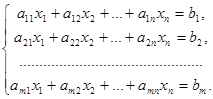
Consider a system of m linear equations with n variables x1, x2, x3, …, xn:
 (1)
(1)
The coefficients aik (i = 1, 2, …, m; k = 1, 2, …, n) of unknowns are enumerated by two indices: the first index i indicates the number of the equation, and the second j – the number of the variable. This numeration of coefficients of the system (1) by two indices is analogous to the numeration of matrix elements. According to the system (1) consider the following matrices:
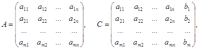


The matrix А is called the basic matrix of the system (1), and the matrix С – the extended one. Multiplying the matrices А and Х we obtain:
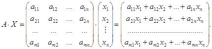
Thus, the system (1) in a matrix representation is written as:
A × X = B (2)
A decision of the system (1) is an ordered set of real numbers (a1, a2, …, an) which inverts each equation of the system in a true numeric identity.
The system of equations (1) is called compatible if it has at least one decision and is called non-compatible if it has no decision.
The system of equations (1) is called determinate if it is compatible and has a unique decision, and is called indeterminate if it is compatible and has infinitely many decisions.
To find a decision of the system of linear equations (1) firstly it is necessary to conduct its investigation which is the following:
1. To clarify whether the given system (1) is compatible or not;
2. If the system is compatible then determine whether it is determinate or indeterminate;
3. If the system is determinate then find its unique decision;
4. If the system is indeterminate then describe an infinite set of its decisions.
Solving a system of linear equations by means of determinants
(Cramer rule)
Consider a system of two equations with two unknowns: 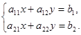 (3).
(3).
The determinant  is called the basic determinant of the system of equations (3), and the determinants
  and
and  are called the
auxiliary determinants of the system (3).
To exclude the variable у, multiply both parts of the first equation on а22, and both parts of the second one on (– а12) and then add these equations termwise. As a result we obtain:
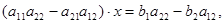 i.e.
i.e. 
To exclude the variable х, multiply both parts of the first equation on (- а21), and the second equation – on а11 and then add the obtained equations termwise. As a result we obtain:
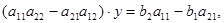 i.e.
i.e. 
Thus, the original system (3) is equivalent to the following:  (4)
(4)
The following cases are possible:
1) D ¹ 0.
In this case each equation of the system (4) has a unique decision:  (5)
(5)
Consequently the original system (3) is compatible and determinate. Its unique decision is founded by the formulas (5) which are called the Cramer formulas.
2) D = 0, but at least one of Dх, Dу is not equal to zero.
In this case there is at least one equation of the system (4) which has no decision. Consequently the original system (3) has no decision, i.e. is non-compatible.
3) D = Dх = Dу = 0.
In this case each equation of the system (4) has infinitely many decisions. Consequently the original system (3) is compatible and indeterminate.
Example 1. Solve the system 
Solution: 1)Compute the basic determinant of the system 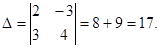 2) Compute the auxiliary determinants of the system:
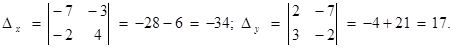
Since D = 17 ¹ 0 then 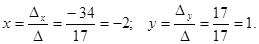
Checking: 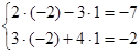 It is true.
The answer: x = -2; y = 1.
The Cramer formulas are fair for such systems of linear equations at which the basic determinant of a system is not equal to zero and the number of variables is equal to the number of equations.
For example, for a system of three linear equations with three variables x, y, z:
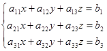
the Cramer formulas are deduced analogously and have the following form:
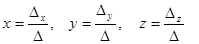 (6)
(6)
where 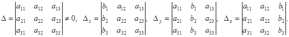
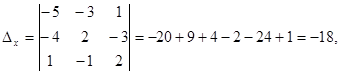
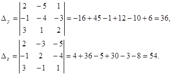
Example 2. Solve the system of equations: 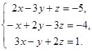
Solution. Compute the basic and auxiliary determinants of the system:
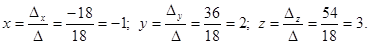
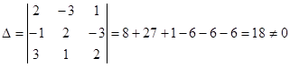 – the system has a unique decision.
Checking: 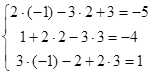 – it is true.
The answer: х = -1; y = 2; z = 3.
Example 3. The shoe factory specializes on producing three kinds: boots, trainers and ankle boots; thus the raw material of three types is used: S1, S2, S3. The norms of expense of each of them per one pair of footwear and the volume of expense of raw material per one day are set by the table:
| Kind of the raw material | Norm of expense of the raw material per one pair in standard units | Expense of the raw material per one day in standard units | ||
| Boots | Trainers | Ankle boots | ||
| S1 | ||||
| S2 | ||||
| S3 |
Find the daily volume of output of each kind of footwear.
Solution: Let the factory producesdaily x1 pairs of boots, x2 pairs of trainers and x3 pairs of ankle boots. Then according to the expense of the raw material of each kind we have the following system:
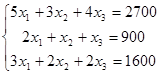
Solving the system by an arbitrary way, we find (200; 300; 200), i.e. the factory produces 200 pairs of boots, 300 pairs of trainers and 200 pairs of ankle boots.
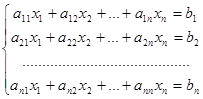
In general case for a system of n linear equations with n variables

the Cramer formulas are the following: 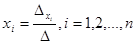 (7)
(7)
where 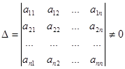 – the basic determinant of the system,
  – the determinant obtained from the basic determinant D by replacement of the i –th column on the column of constant terms.
Inverse matrix
Consider a system of n linear equations with n variables (x1, x2, …, xn):
 (8)
(8)
Consider 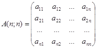 ,
,  and
and 
Then the system (8) is written in a matrix representation:
A(n; n)× X(n; 1) = B(n; 1) (9)
A matrix A(n; n) is called regular if its determinant is not equal to zero, i.e. 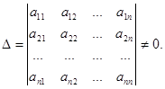
A matrix A-1(n; n) is called inverse to a matrix A(n; n) if the product
A(n; n) ×A-1(n; n)= A-1(n; n)×A(n; n) = E(n; n),
where 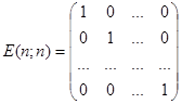 is the identity matrix.
Find a decision of the matrix equation (9), i.e. find a matrix-column of variables X(n; 1). Multiply both parts of the matrix equation (9) on the left (since the order of multiplying matrices is important) on matrix A-1(n; n). As a result we obtain:
A-1× (A× X) =A-1× B or (A-1× A)× X = A-1× B; E× X = A-1× B, but E× X = X, consequently X = A-1× B. (10)
Thus, we find a decision (matrix X(n; 1)) of the matrix equation by formula (10), i.e. to find matrix X(n; 1) (and variables x1, x2, …, xn) it is necessary to find an inverse matrix A-1(n; n) and multiply it on matrix B(n; 1). Consequently all is reduced to a determination of an inverse matrix A-1(n; n).
Show a finding the inverse matrix А-1 on example of a system of three linear equations with three unknowns: 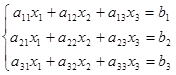 .
.
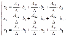
Let 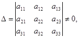 then the system has a unique decision which is computed by the Cramer formulas:
 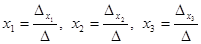 .
.
Transform the auxiliary determinants of the system:
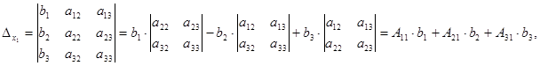
where А11, А21, А31 – the cofactors of the elements а11, а21, а31 of matrix 
Transforming analogously the second and the third formulas, we finally obtain:
 This implies:
 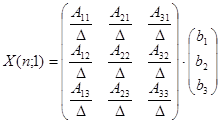 (11)
(11)
We obtain the rule of finding the inverse matrix by formulas (10) and (11):
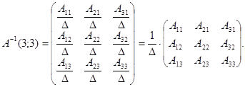 (12)
(12)
It is necessary to mark that the inverse matrix exists only for regular matrixes (i.e. for square matrixes at which the determinant is not equal to zero).
The order of actions for finding the inverse matrix А-1 to a matrix А is the following:
1) Compute the determinant D of the matrix А (if it equals zero then there is no inverse matrix).
2) Compute the cofactors Aij to all the elements aij of the matrix А.
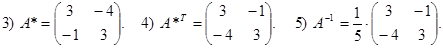
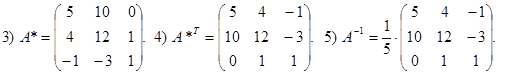
3) Compose the matrix A * of the cofactors.
4) Compose the matrix A*T – transposed to the matrix A * (a matrix obtained from the matrix A * by interchanging rows and columns is called transposed to the matrix A *).
5) Each element of the matrix A*T is divided on the determinant D ¹ 0.
Thus, finally we have 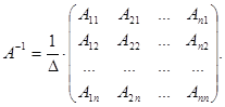
Example 3. Find the inverse matrix to the matrix 
Solution. 1) 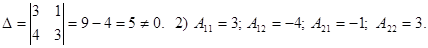
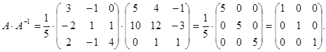
Checking:

Example 4. Find the inverse matrix to the matrix 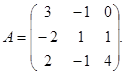
Solution: 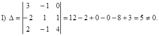
2) А11 = 5; A12 = 10; A13 = 0; A21 = 4; A22 = 12; A23 = 1; A31 = -1; A32 = -3;
A33 = 1.
Checking: