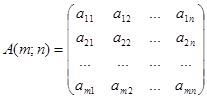
Consider a matrix of the dimension  :
: 
Take a natural number k such that k £ m and k £ n. Choose in A arbitrary k rows and k columns. As a result we obtain a square matrix of the k -th order. The determinant of this matrix is called minor of the k -th order of the matrix A. The number of all minors of different orders can be great even for a matrix of non-large dimension. For example, a matrix of dimension 4 x 5 has 5 minors of the fourth order, 40 minors of the third order, 60 minors of the second order and 20 minors of the first order (minors of the first order coincide with elements of a matrix).
The rank of a matrix A is the greatest order of its non-equal to zero minors. The rank of a matrix is denoted by Rank A or r(A).
This definition implies that for calculation of the rank of a matrix it is necessary to compute all minors of all orders of a matrix A, choose non-equal to zero minors and determine which one of them has the greatest order. However such a method of calculating the rank of a matrix is useless due to a great number of calculations because there can be a lot of minors at a matrix. For example, a matrix A(4; 5) has 125 minors.
Thus, a question on a shorter method of calculating the rank of a matrix emerges. One of such methods is based on the theorem on bordering:
Theorem. If there is a non-equal to zero minor of the r -th order in a matrix A and all its bordering minors of the r+ 1-th order are equal to zero then the rank of A is equal to r, i.e. r(A)=r.
The theorem implies a practical rule of calculating the rank of a matrix: find a minor M ¹ 0 in a matrix A and compute all its bordering minors. If all of them are equal to zero then the rank of the matrix is equal to the order of minor M. If for calculating process of bordering minors we find a non-equal to zero minor M* then we interrupt further calculating the bordering minors and pass to a bordering the minor M*, i.e. repeat the described cycle of calculations. There will be finitely many such cycles and the number of such cycles doesn’t exceed maximal of m and n, i.e. the number of rows and the number of columns.
Example 1. Calculate the rank of matrix 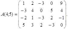
Solution: Consider, for example, the minor 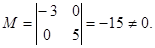 This implies Rank A ³ 2. Further take three minors of the third order M1, M2 and M3 which are bordering the minor M:
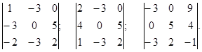
Calculate 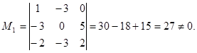
Consequently, Rank A ³ 3. Since M1 ¹ 0 it isn’t necessary to calculate the rest two bordering minors. Now we will consider bordering minors of the fourth order for the minor M1:
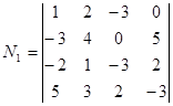 and
and 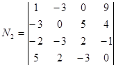 .
.
Since N1=31¹ 0 then Rank A ³ 4 and it isn’t necessary to calculate the minor N2. And since there is no minor of the fifth order in the matrix A then Rank A = 4.
The considered methods of calculating the rank of a matrix (based on just the definition and the theorem on bordering) are practically useless for matrices of higher orders due to a great number (complexity) of calculations. Therefore, we formulate a theorem permitting to calculate the rank of a matrix of an arbitrary order by a universal method.
Theorem. The rank of a matrix doesn’t change if:
1) All the rows are replaced by the corresponding columns and vice versa;
2) Replace two arbitrary rows (columns);
3) Multiply (divide) each element of a row (column) on the same non-zero number;
4) Add to (subtract from) elements of a row (column) the corresponding elements of any other row (column) multiplied on the same non-zero number.
Example 2. Calculate the rank of a matrix 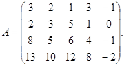
Solution: 1) Multiply all the elements of the last column on (-1) and replace the last and the first columns, and we obtain: 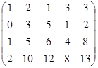 .
.
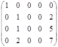
2) Add to all the elements of the third row the corresponding elements of the first row multiplied on (-1), and we obtain: 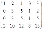 .
.
3) Add to all the elements of the fourth row the corresponding elements of the first row multiplied on (-2), and we obtain: 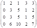 .
.
As a result, we obtained “good” first column (it consist of one 1 and zeros). Further we make zeros in the first row by this column.
4) Add to all the elements of the second column the corresponding elements of the first column multiplied on (-2); subtract from the elements of the third column the corresponding elements of the first column; add to all the elements of the fourth column the corresponding elements of the first column multiplied on (-3); add to all the elements of the fifth column the corresponding elements of the first column multiplied on (-3). The rank of the matrix A will not change after these transformations. As a result, we have: 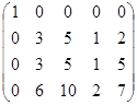 .
.
5) The elements of the second and the third columns can be reduced on common for them non-zero multipliers (3 and 5 respectively). We have: 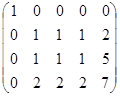 . We see that there are three identical columns in the matrix (second, third and fourth). Subtract from the elements of the third and the fourth columns the corresponding elements of the second column, and we obtain:
 .
.
6) Add to all the elements of the fifth column the corresponding elements of the second column multiplied on (-2), and we obtain: 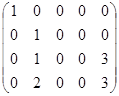 .
.
As a result, we have “good” second row (it consists of one 1 and zeros). Further, subtract from the elements of the third row the corresponding elements of the second row; add to all the elements of the fourth row the corresponding elements of the second row multiplied on (-2), and we obtain: 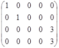 . We see that there are two identical rows in the matrix. Subtract from the elements of the fourth row the corresponding elements of the third row, and we obtain:
 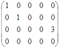 .
.
Interchange the third and the fifth columns and reduce the elements of the third column on common multiplier 3, and finally we obtain: 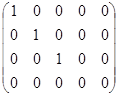 . Consequently, Rank A = 3.
The notion of the rank of a matrix is used for investigation of compatibility of a system of linear equations.
Consider a system of m linear equations with n variables x1, x2, x3, …, xn:
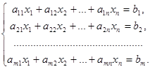
The basic and extended matrices of the system are the following:
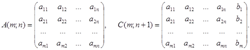
A criterion for compatibility of a system of linear equations is expressed by the Kronecker-Capelli theorem. This theorem gives an effective method permitting in finitely many steps to determine whether the system is compatible or not.
Theorem of Kronecker-Capelli. A system of linear equations is compatible iff the rank of the basic matrix A equals the rank of the extended matrix C, i.e. Rank A = Rank C. Moreover:
1) If Rank A = Rank C = n (where n is the number of variables in the system) then the system has a unique decision.
2) If Rank A = Rank C < n then the system has infinitely many decisions.
Solving a system of linear equations by the Gauss method
It is convenient to produce a numerical solution of linear algebraic equations by determinants for systems of two and three equations. And in case of systems of a greater number of equations it is much more profitable to use the Gauss method which consists of a sequential (successive) elimination of unknowns.
Let's explain the sense of this method on a system of fours equations with fours unknowns:
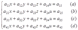
Suppose that а11 ¹ 0 (if а11 = 0 then we change the order of equations by choosing as the first equation such an equation in which the coefficient of х is not equal to zero).
I step: divide the equation (а) on а11, then multiply the obtained equation on а21 and subtract from (b); further multiply (а)/a11 on а31 and subtract from (с); at last, miltiply (а)/a11 on а41 and subtract from (d).
As a result of I step, we come to the system
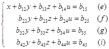
where bij are obtained from aij by the following formulas:
b 1 j = a 1 j / a 11 (j = 2, 3, 4, 5);
bij = aij – ai 1 × b 1 j (i = 2, 3, 4; j = 2, 3, 4, 5).
II step: do the same actions with (f), (g), (i) (as with (a), (b), (c), (d)) and etc.
As a final result the initial system will be transformed to a so-called step form:
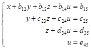
From a transformed system all unknowns are determined sequentially without difficulty. If the system has a unique solution, the step system of equations will be reduced to triangular in which the last equation contains one unknown. In case of an indeterminate system, i.e. in which the number of unknowns is more than the number of linearly independent equations and therefore permitting infinitely many solutions, a triangular system is impossible because the last equation contains more than one unknown. If the set of equations is incompatible then after reduction to a step form it contains at least one equation of the kind 0 = 1, i.e. the equation in which all unknowns have zero factors, and the right part is not equal to zero. Such system has no solutions.
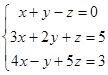
Example 1. 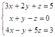
Interchange the first and the second equations of the system:
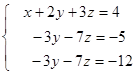
Subtract from the second equation the first equation multiplied on 3; also subtract from the third equation the first equation multiplied on 4. We obtain:
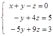
Further subtract from the third equation the second equation multiplied on 5:
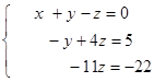
Multiply the second equation on (-2), and the third – divide on (-11):
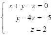
The system of equations has a triangular form, and consequently it has a unique decision. From the last equation we have z = 2; substituting this value in the second equation, we receive у = 3 and, at last from the first equation we find х = -1.
Example 2. 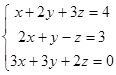
Subtract from the second equation the first equation multiplied on 2; also subtract from the third equation the first equation multiplied on 3:
Further subtract from the third equation the second equation and we obtain:
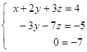
We have the equation 0 = -7. Consequently the system has no decision.
Example 3. 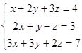
Subtract from the second equation the first equation multiplied on 2; also subtract from the third equation the first equation multiplied on 3:
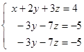
Further subtract from the third equation the second equation and we obtain:
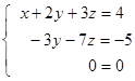
We have that unknowns are more than equations. Express х and у through the variable z:
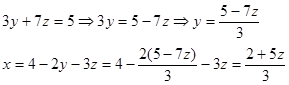
As a result we have:  , where z is an arbitrary number.
Thus, the system has infinitely many decisions.
Glossary
compatible – совместный; determinate – определенный
basic – основной; auxiliary – вспомогательный
boots – сапоги; trainers – кроссовки; ankle boots – ботинки
inverse matrix – обратная матрица
regular matrix – невырожденная матрица; rank – ранг
to border – окаймлять; triangular – треугольный
sequential (successive) – последовательный
Exercises for Seminar 3
3.1. Solve systems of linear equations: a)  ; b)
; b)  ;
;
c)  ; d)
; d) 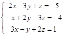 ; e) ; f)
 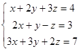 .
.
3.2. Find the inverse matrix  to the matrix
3.3. Find the inverse matrix to the matrix 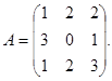
3.4. Find the inverse matrix  to the matrix
3.5. Find the ranks of matrices:
a)  b)
b)  c)
c)  ; d)
; d) 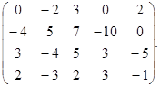
3.6. Determine the compatibility of the following system of equations by the Kronecker-Capelli theorem: 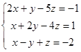 .
.